
Project information
- Category: Deep Learning
- Co-Authors: Rui Shen, Rongguang Wang
- Project date: Dec, 2019
- Github: https://github.com/Sherry-SR/dl_graph_connectomes
Abstract
Brain connectomes is a comprehensive map that shows the structural and functional connectivity of neural pathways in the human brain. Analyzing the information encoded by connectomes can promote a critical understanding of the early diagnosis of many neuropsychiatric disorders, such as Autism Spectrum Disorder (ASD). Brain connectomes data is usually represented as a graph with a connectivity matrix illustrating the strength of neural connections (e.g. temporal correlation of brain activities) between brain regions. In contrast to classical graph analysis methods that depend on hand-engineering descriptors, recent progress of extending deep learning approaches to non-grid data have opened new opportunities for building predictive models for brain connectomes in a data-driven learning fashion. However, due to the existence of large noise and limited training samples, directly applying a deep network is prone to over-fitting. In this work, we present a novel graph convolutional neural network (GCN) with node-wise batch normalization and embedding normalization 1 for better generalization. We performed experiments on the ABIDE dataset and achieved state-of-the-art 68.7% classification accuracy.
Method
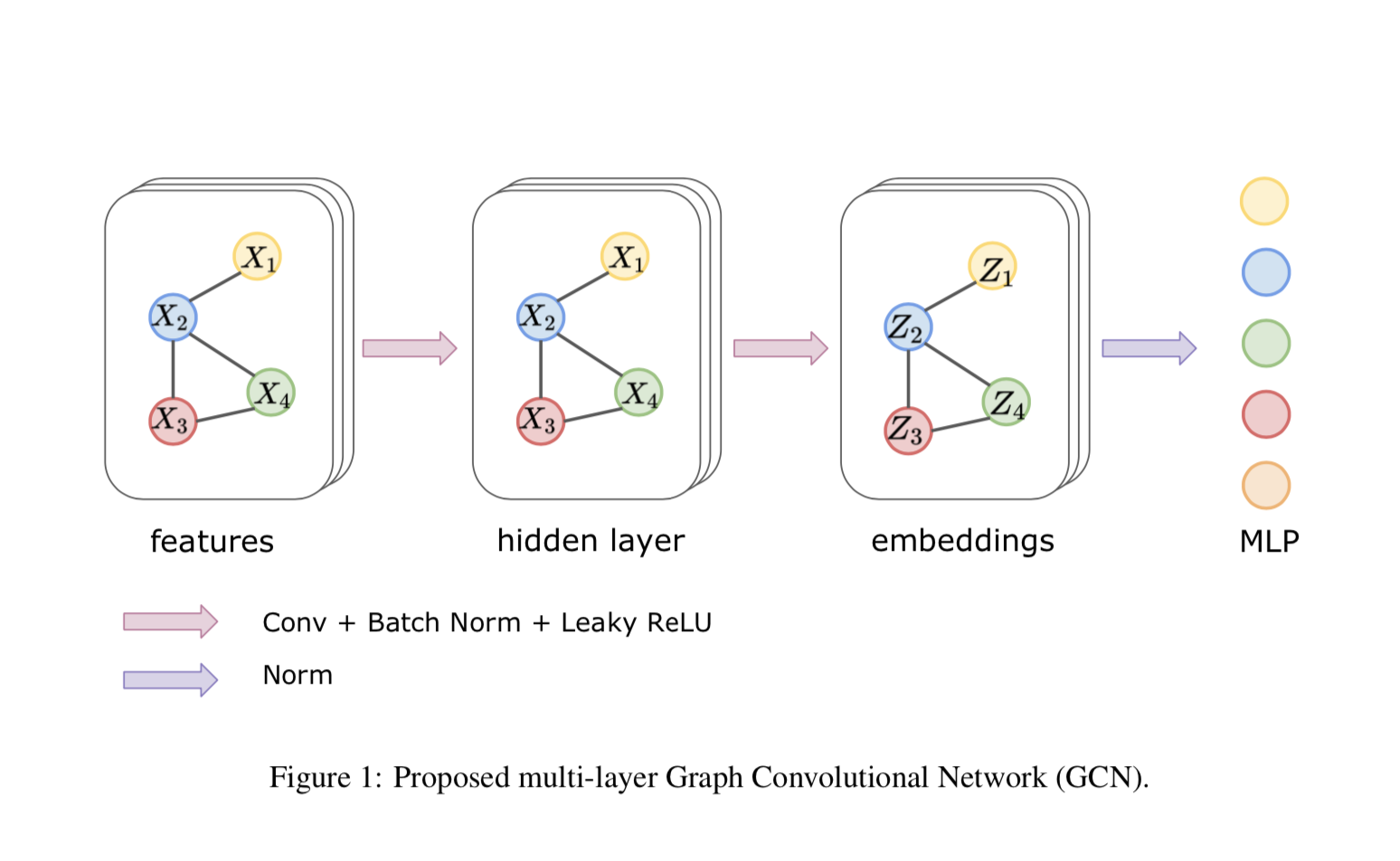
In this section, we described our approach for classifying subjects with ASD. Figure 1 illustrates an overview of the proposed approach for ASD classification. In the proposed method, we used the first-order approximation of GCN in the first stage to obtain embedding for a graph, and a multi-layer perceptron (MLP) in the second stage for the classification task. Multiple normalization tricks were used to improve the stability in the training process and achieve better generalization. A Dropout layer was used between MLP to prevent further over-fitting.
CNNs enable extraction of statistical features from grid-structured data, in the form of local stationary patterns, and their aggregation for different semantic analysis tasks, e.g. image recognition [6]. When the signal of interest does not lie on a regular domain, e.g. graphs, direct application of CNNs might be problematic due to the presence of convolution and pooling operators which typically defined on grids. Generalizing the convolution to graphs is a common way to address this problem.
Two types of novel normalization layers were used to help the stability and convergence in the training process. Between each graph convolutional layer, a normalization layer was used to reduce the “covariate shift” for each node. Unlike traditional batch normalization which normalizes the summed inputs to each channel over the training cases, node normalization applies a similar operation but for each node in the graph. It can be formulated as
\begin{equation} \tilde{x}_{i, j}^{v}=\frac{x_{i, j}^{v}-E_{i \in \mathcal{B}, j \in \mathcal{C}}\left[x_{i, j}^{v}\right]}{\sqrt{\operatorname{Var}_{i \in \mathcal{B}, j \in \mathcal{C}}\left[x_{i, j}^{v}\right]}} \times \gamma^{v}+\beta^{v} \end{equation}where \(\mathcal{B}\) and \(\mathcal{C}\) contains indices for each sample in the mini-batch and each channel of the filters respectively. The node normalization has similar advantages as batch normalization, such as enabling a higher learning rate and regularizing the model. Additionally, as the graph embedding is generated in the form of nodes, node normalization which balances the nodes of the graph can improve the stability and efficiency in extracting embedding.
Another normalization layer was applied between GCN and MLP for each sample over the dimension of graph embedding, which is defined as
\begin{equation} \tilde{x}_{i}^{k}=\frac{x_{i}^{k}-E_{k \in \mathcal{K}}\left[x_{i}^{k}\right]}{\sqrt{\operatorname{Var}_{i \in \mathcal{K}}\left[x_{i}^{k}\right]}} \end{equation}where \(\mathcal{K}\) stands for the embedding dimensions. This normalization is actually equivalent to layer normalization or instance normalization when input size equals to 1. This layer can act like contrast normalization over the embedding. It can stabilize the hidden state dynamics and keep characteristics for an individual sample at the same time. No running average needs to be calculated during training, and large noise in one sample will not affect each other in the mini-batch.
Data Set
The Autism Brain Imaging Data Exchange (ABIDE) - ABIDE is a multi-site dataset openly sharing anatomical and functional brain imaging data of 539 individuals diagnosed with Autism Spectrum Disorder (ASD), as well as 573 normal controls (NC). We used the data processed by the Configurable Pipeline for the Analysis of Connectomes (CPAC). This pipeline performs motion correction, global mean intensity normalization and standardization of fMRI data to MNI space
Functional Connectomes - Functional connectomes were generated by first averaging rs-fMRI time series for each ROI, then calculating the temporal Pearson correlation coefficients between each pair of averaged fMRI signals.
Experiments
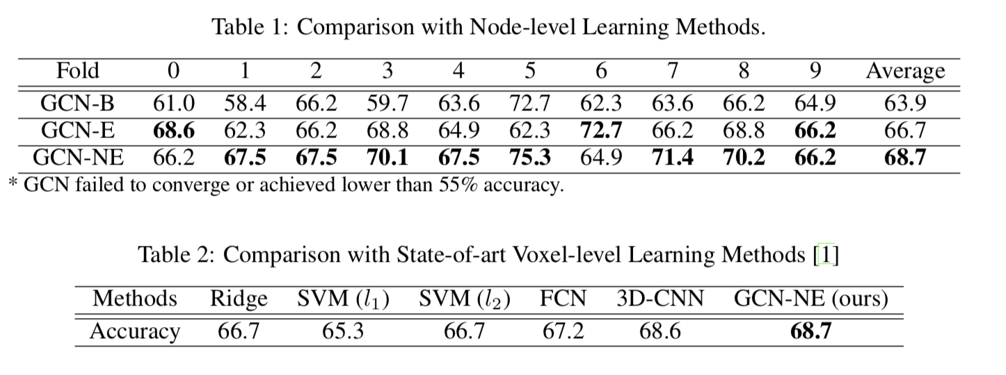
In our experiments, we performed a node-level connectomes-based classification task of ASD v.s. NC using 4 deep learning frameworks: GCN, GCN with batch normalization (GCN-B), GCN with embedding normalization (GCN-E), and GCN with both node and embedding normalization (GCN- NE). We conducted 10-fold cross-validation on the ABIDE dataset. Results are also compared with other state-of-art voxel-level learning methods.
Results
Table 1: Comparison with Node-level Learning Methods. \begin{array}{cccccccccccc} \hline \text { Fold } & 0 & 1 & 2 & 3 & 4 & 5 & 6 & 7 & 8 & 9 & \text { Average } \\ \hline \hline \text { GCN-B } & 61.0 & 58.4 & 66.2 & 59.7 & 63.6 & 72.7 & 62.3 & 63.6 & 66.2 & 64.9 & 63.9 \\ \hline \text { GCN-E } & \mathbf{6 8 . 6} & 62.3 & 66.2 & 68.8 & 64.9 & 62.3 & \mathbf{7 2 . 7} & 66.2 & 68.8 & \mathbf{6 6 . 2} & 66.7 \\ \hline \text { GCN-NE } & 66.2 & \mathbf{6 7 . 5} & \mathbf{6 7 . 5} & \mathbf{7 0 . 1} & \mathbf{6 7 . 5} & \mathbf{7 5 . 3} & 64.9 & \mathbf{7 1 . 4} & \mathbf{7 0 . 2} & \mathbf{6 6 . 2} & \mathbf{6 8 . 7} \\ \hline \end{array} Table 2: Comparison with State-of-art Voxel-level Learning Methods \begin{array}{ccccccc} \hline \text { Methods } & \text { Ridge } & \text { SVM }\left(l_{1}\right) & \text { SVM }\left(l_{2}\right) & \text { FCN } & \text { 3D-CNN } & \text { GCN-NE (ours) } \\ \hline \hline \text { Accuracy } & 66.7 & 65.3 & 66.7 & 67.2 & 68.6 & \mathbf{6 8 . 7} \\ \hline \end{array}